Beyond Statistics Histogram – Part 1

In this article I will start to examine estimations and execution plans for queries that compare values in columns with literal values which are beyond the statistics histogram for that column. The problem is also known as key ascending column statistics problem.

As in previous posts we remain here conservative regarding sample tables. We’ll create again our Orders table and populate it with 10M rows. All orders will have the order date from 1998 to 2013. In addition we’ll create one index on the custid and orderdate columns. Use the following link to download the code to create and populate the table.

Please be aware that above script will run few minutes and will create a table with the size about 1.5 GB and almost 500M for two indexes.

Since we have created indexes after the table population at this point statistics are up to date. And only at this point. As soon as data changes or new orders are inserted into the table, statistics are out of date; thus they are always out of date, at least for volatile tables. That means that most recent orders are not seen by statistics objects. Can this causes a serious problem? Yes, for statistics on columns where most of newly added rows has value which is greater than the maximum value from the statistics histogram for this column. If values are monotonically increasing these columns are called key ascending columns. For example transaction date, insert timestamp, sequence number column are typical key ascending columns.

Let’s back to our table and simulate this behavior. We’ll insert another 1M rows into the Orders table. For all orders we’ll put some order date from 2014, so that all of them have value which is greater than the maximum value from the statistics histogram. The code you can get here. Please note that order dates are populated random and the column is not key ascending column, it just met the above criteria that newly added rows have value which is greater than the maximum value from the statistics histogram on the order date column.

One million of rows is a large number but still not enough to trigger automatic statistics update. Therefore our statistics object is still the same as it was after initial load:

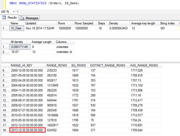
The most recent order for the statistics histogram is still 30^th December 2013, although we added 1M rows after that!

Now we need to execute some common queries against such table. For instance let’s help our customer with the ID 160 to find all his or her orders from 2014! This is a pretty easy task, isn’t? Some our customers would also know how to write such simple query:

SELECT * FROM dbo.Orders
WHERE custid = 160 AND orderdate >= '20140101' AND orderdate < '20150101';

A simple query with two predicates; we have an index on both of them. Imagine that our customer is a typical customer (i.e. his number of orders is not far away from the average number of orders). We expect fast response time, in the execution plan we expect to see an Index Seek on the index on the customer id and not too much logical reads (<10K in this case).

What we get?

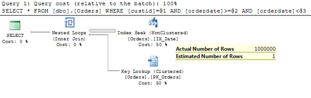
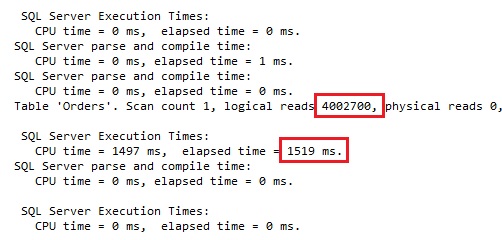
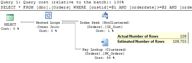
Ooops… Elapsed time 1.5 seconds! More than 4 millions of logical reads!? Only one expectation is met: the plan contains an Index Seek operator. Unfortunately on the “wrong” index. In the plan we can see that the query engine takes all orders from 2014 and then (in the Key Lookup operator) checks if an order has been made by the customer 160. Opposite to what we expected! We have expected that the QO will first get all orders for customer 160 and then extract those from 2014. It’s very uncommon, even impossible, that one customer has more orders than all customers for a whole year. It is more efficient to get rid of most of the orders in the first step and then in a second step to execute the other filter. That’s how we think it should work. That’s exactly how it works! Where is the problem then?

How SQL Server in this case decides should an index or which one from two indexes will be used? It estimates selectivity of individual predicates and then according to selectivity makes a decision. If two much rows will be returned it will not use an index at all. Otherwise it will use the index on the column with higher selectivity. Let’s decompose our query to two queries with individual predicates and choose Display Estimated Execution Plan.

SELECT * FROM dbo.Orders WHERE custid = 160;
SELECT * FROM dbo.Orders WHERE orderdate> = '20140101' AND orderdate < '20150101';

Here is the result:

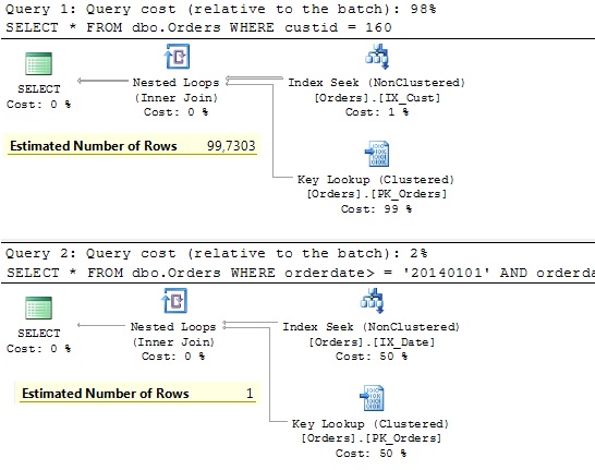
Now it’s clear why SQL Server decided to use the index on the order date column. It expected only one row! Actually it did not expect rows at all, but when SQL Server does not expect rows it returns 1 and not 0. This is strange behavior and has something to do with basic assumptions in the old cardinality estimator.

So, 1 is less than 100 and therefore it makes more sense to use the index on the orderdate than one on the custid. Of course, this is great when estimations are more or less correct, but in this case the one with orderdate is significantly wrong. The only problem with it is that SQL Server does not know it. It does not know for any order from 2014 although we are in November 2014! This is very danger as we can see from the execution plan. Almost 2 seconds and 4 Mio logical reads. And imagine that you have 10K customers logged in the system where 100 of them check their recent orders…

OK, it’s clear that default behavior in SQL Server 2012 leads to serious problems with significant performance issues.

Let’s see what happens when we execute the same query against SQL Server 2014 with the database compatibility level 120.

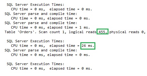
The elapsed time dropped to 26 milliseconds! Instead of millions of loaded pages only 455 logical reads were needed now. And an Index Seek against the “right” column. Impressive! New cardinality estimator rocks!

Let’s look at the estimation process in the new CE. We’ll display again the estimated execution plan for individual predicates as we did for SQL Server 2012. Here is the result:

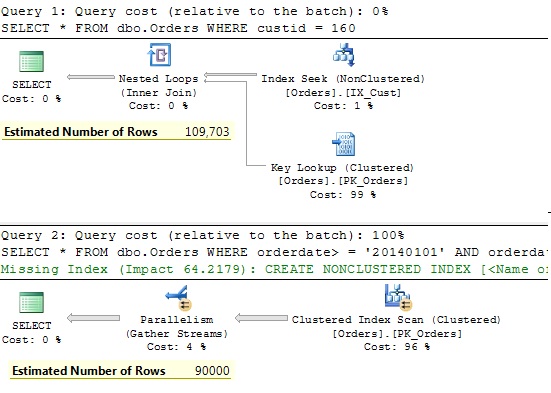
New CE expects significantly more rows for the date predicate (90K compared to old CE’s 1) and the query optimizer had to make an easy decision and to use an Index Seek on the customer id. The new CE stills underestimates the number of rows; the actual number is 1M, but to solve the estimation problem for this query pattern it was enough to get rid of truly underestimations of 1 row. It’s enough (in this particular case) to estimate for instance 200 rows and the expected index would be used. The new CE comes up with 90K and solved the problem. In one of our next posts we will look more detailed in this estimation. You will see the other side of the medal of the new CE.

One our predicate (orderdate) has been affected with outdated statistic, the other predicate wasn’t affected. However, from the estimated plans you can see that the estimated number of rows is not the same for old and new CE. The old CE estimates 99.7 while the new CE comes with a little bit more 109.7. A “little bit” is 10% in this case. A detailed explanation about this change in the new CE you can find in my previous post.

Conclusion

New CE solves problems for queries with large tables which are caused by conservative and hardcoded underestimation done by the old CE (1). It estimates significantly more and therefore avoid the problem we described here. However, as we mentioned the way how new CE estimates is good enough to avoid this problem, there are some other query patterns too. We’ll cover them in the next posts.

Thanks for reading.